LaTeX's features for typesetting mathematics make it a compelling choice for writing technical documents. This article shows the most basic commands needed to get started with writing maths using LaTeX.
Writing basic equations in LaTeX is straightforward, for example:
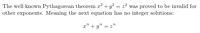
\documentclassarticle> \begindocument> The well known Pythagorean theorem \(x^2 + y^2 = z^2\) was proved to be invalid for other exponents. Meaning the next equation has no integer solutions: \[ x^n + y^n = z^n \] \enddocument>
As you see, the way the equations are displayed depends on the delimiter, in this case \[. \] and \(. \) .
L a T e X allows two writing modes for mathematical expressions: the inline math mode and display math mode:
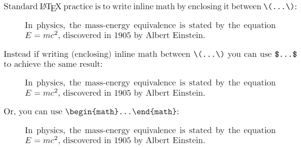
You can use any of these "delimiters" to typeset your math in inline mode:
They all work and the choice is a matter of taste, so let's see some examples.
\documentclassarticle> \begindocument> \noindent Standard \LaTeX<> practice is to write inline math by enclosing it between \verb|\(. \)|: \beginquote> In physics, the mass-energy equivalence is stated by the equation \(E=mc^2\), discovered in 1905 by Albert Einstein. \endquote> \noindent Instead if writing (enclosing) inline math between \verb|\(. \)| you can use \texttt\$. \$> to achieve the same result: \beginquote> In physics, the mass-energy equivalence is stated by the equation $E=mc^2$, discovered in 1905 by Albert Einstein. \endquote> \noindent Or, you can use \verb|\beginmath>. \endmath>|: \beginquote> In physics, the mass-energy equivalence is stated by the equation \beginmath>E=mc^2\endmath>, discovered in 1905 by Albert Einstein. \endquote> \enddocument>
Use one of these constructions to typeset maths in display mode:
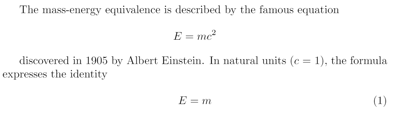
Display math mode has two versions which produce numbered or unnumbered equations. Let's look at a basic example:
\documentclassarticle> \begindocument> The mass-energy equivalence is described by the famous equation \[E=mc^2\] discovered in 1905 by Albert Einstein. In natural units ($c$ = 1), the formula expresses the identity \beginequation> E=m \endequation> \enddocument>
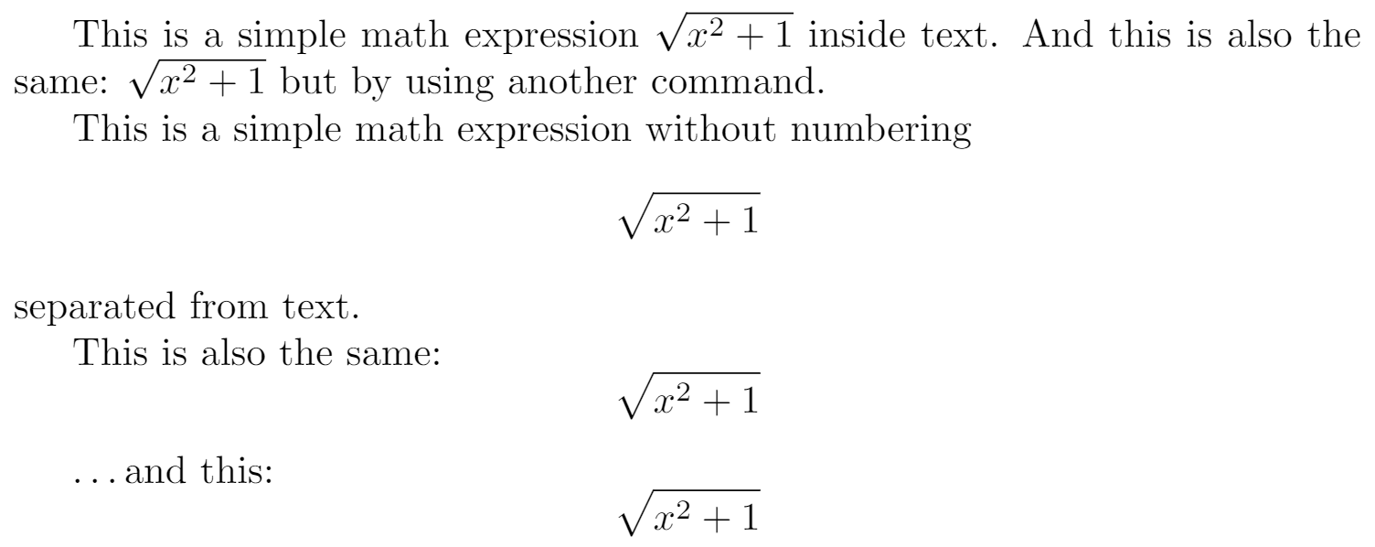
The following example uses the equation* environment which is provided by the amsmath package—see the amsmath article for more information.
\documentclassarticle> \usepackageamsmath> % for the equation* environment \begindocument> This is a simple math expression \(\sqrt2+1>\) inside text. And this is also the same: \beginmath> \sqrtx^2+1> \endmath> but by using another command. This is a simple math expression without numbering \[\sqrt2+1>\] separated from text. This is also the same: \begindisplaymath> \sqrtx^2+1> \enddisplaymath> \ldots and this: \beginequation*> \sqrtx^2+1> \endequation*> \enddocument>
Below is a table with some common maths symbols. For a more complete list see the List of Greek letters and math symbols:
| description | code | examples |
|---|---|---|
| Greek letters | \alpha \beta \gamma \rho \sigma \delta \epsilon | $$ \alpha \ \beta \ \gamma \ \rho \ \sigma \ \delta \ \epsilon $$ |
| Binary operators | \times \otimes \oplus \cup \cap | × ⊗ ⊕ ∪ ∩ |
| Relation operators | < >\subset \supset \subseteq \supseteq | < >⊂ ⊃ ⊆ ⊇ \subset \ \supset \ \subseteq \ \supseteq > |
| Others | \int \oint \sum \prod | ∫ ∮ ∑ ∏ |
Different classes of mathematical symbols are characterized by different formatting (for example, variables are italicized, but operators are not) and different spacing.
The mathematics mode in LaTeX is very flexible and powerful, there is much more that can be done with it: